As we commented in previous posts of this blog, Machine learning (#ML) is a subset of techniques within the concept of #ArtificialIntelligence that allow machine to perform activities to which to which they have not been programmed to. This programming bases on the type of data available and the labels of this data.
In this post we will review some important concepts or prediction models inside Machine Learning that are considered the initiators of what now we know as Convolutional Neural Networks (CNNs).
One of the earliest concepts that appeared is the “Decision Tree”. This type of “algorithm” is a supervised method that represents all the possible decisions of a particular problem and their consequences. It is normally used in simple tasks such as the one in the Figure 1, where the Decision Tree tries to illustrate the probability for a customer to receive a loan in a specific bank.

Figure 1: Decision tree example [1]
In this case, depending on some variables such as income or credit history the whole decision tree can be drawn. Once this is done, depending on the type of data we have (in this case, the type of customers this bank has), we will be able to detect the probability of all the possible scenarios.
To know which variables we shall attend to to draw our tree, there are some techniques when processing the input data that tell us, for example, which shall be our main node (or first decision). In this sense, one typical indicator of the main node is the class or column which has less entropy [2].
Decision tree have proven to be very useful in some scenarios. However, they are not very suited for cases in which we have large amount of data. For this reason, the concept of “random forest” appeared, which is nothing else that a set of decision trees to illustrate a large set of questions and consequences. A random forest combines the output of several decision trees in parallel (generated randomly) to generate a final output, [1].
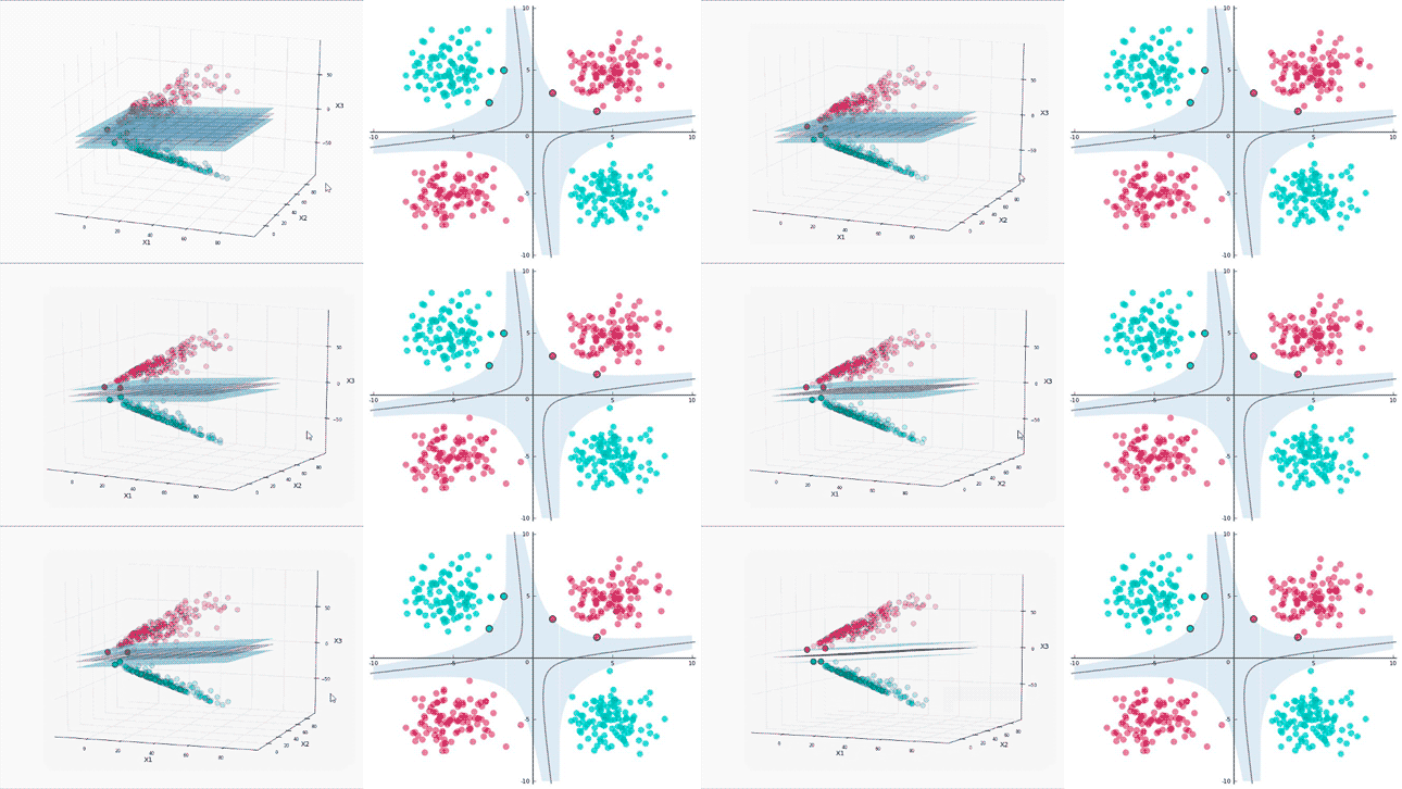
One important set of techniques that appeared a bit after and is meant for classifying or predicting new data samples based on previous training data are the Support Vector Machines (SVM). The #SVM is a supervised learning algorithm that aims to precisely classify an unknown data point in one class or another based on the available training classes.
SVMs group sets of data based on similarities so that it can provide the hyperplane that separates all these sets. Through this, when a new data point comes, depending on its relative position to the hyperplane we could predict to which class it belongs to.

Figure 2: Illustration of a SVM, [3].
Since there are several hyperplanes that can separate the different classes there are two conditions that the hyperplane shall fulfill to be considered the “best” option:
1. It shall separate the data correctly.
2. The distance between the closest data point and the point shall be the maximum.

Figure 3: How to calculate SVMs, [3].
A more powerful concept that #SVM appeared some years later and we already discussed about it in this blog. This is the convolutional neural networks, which are simplified mathematical representations of biological neural networks which communicate between each other to learn patterns or key-features from the input training data.
The CNNs base on convolutions which are mathematical operations in which a function “slides” over time through another function to produce a third one. When processing images, we say that a function or kernel slides over the input function or image to produce a third function or feature map.
Most of layers of a #CNN base on convolution operations. Each layer is in charge of looking for a key feature in the image.

Figure 4: Results of typical convolutions applied on images, [4].
To get an instant and intuitive understanding on how #CNN work, we recommend going to “https://playground.tensorflow.org/”and playing around with the available training data, initialization forms and type of layers. It illustrates the impact of the initial training data and the number of hidden layers, e.g., on the prediction accuracy. Moreover, it gives a representation of the type of features that are being learned by each neuron in the hidden layers, which finally produce the output.

Figure 5: Example of https://playground.tensorflow.org/.
LINKs and references:
